Single Experiment pages
In a single Experiment page, you can visualize and explore all the data you have collected in your training runs. This includes automatically logged and custom metrics, code, logs, text, images, and audio. There are also powerful features available in an Experiment page, such as the Confusion Matrix.
This page describes more advanced procedures you can perform in Experiment pages in the Comet UI. Basics on Experiments are covered in Find your way around: Experiments.
Edit an Experiment name
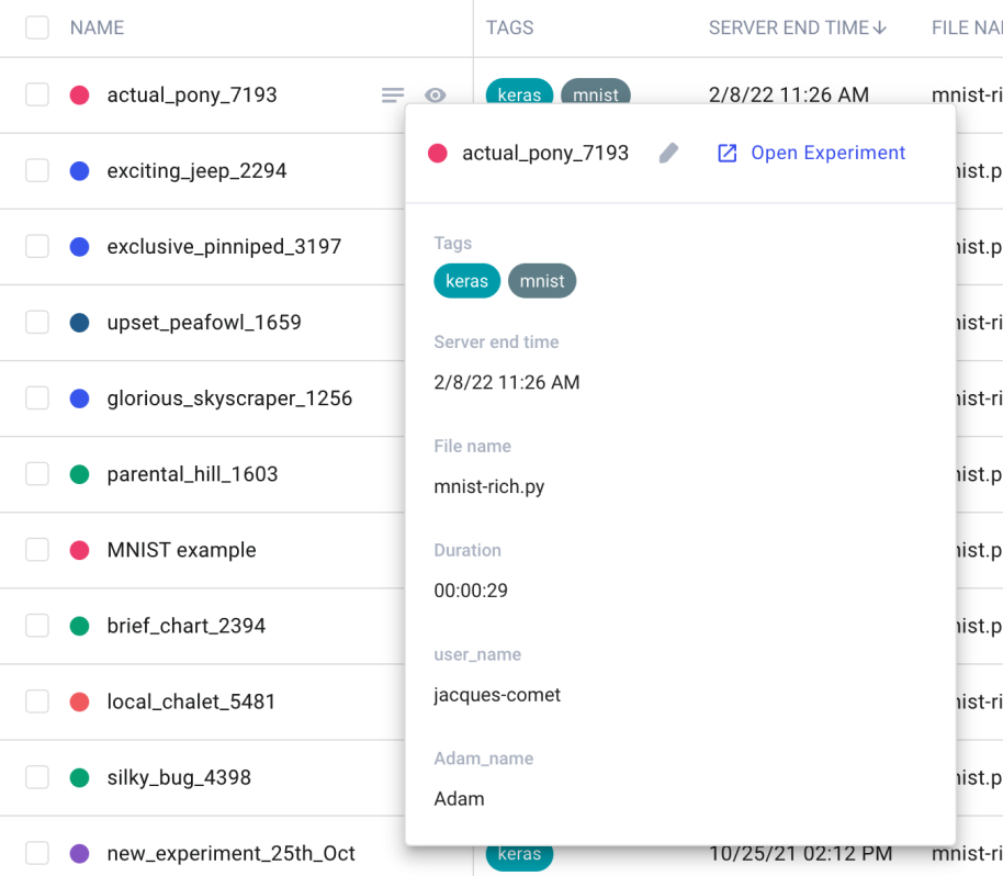
By default, Experiments are given a random ID for a key. You can rename the experiment so that it has a more readable form:
- Hover over the Experiment name.
- Click the Show metadata icon.
- Hover over the Experiment name in the window that opens.
- Click the pencil icon, enter a name, then click the check mark to save the change.
Experiment tabs
Each Experiment contains a set of tabs where you can view additional details about the Experiment. Following is a description of some of the more interesting tabs:
Charts tab
Charts shows all of your charts for this experiment. You can add as many charts as you like by clicking Add Chart. As in the Project view, you can set and save it, set the smoothing level, X axis, Y axis transformation, and how to handle outliers.
For many machine learning frameworks (such as TensorFlow, fastai, PyTorch, scikit-learn, MLflow, and others) many metrics and hyperparameters are automatically logged for you. However, you can also log any metric, parameter, or other value using the following methods:
Code tab
The Code tab contains the source code of the program used to run the Experiment. Note that this is only the immediate code that surrounds the Experiment() creation. In other words, the script, Jupyter Notebook, or module that instantiated the Experiment.
Info
If you run your experiment from a Jupyter-based environment (such as ipython, JupyterLab, or Jupyter Notebook), the Code tab contains the exact history that was run to execute the Experiment. In addition, you can download this history as a Jupyter Notebook under the Reproduce button on the Experiment view. See more here.
Hyperparameters tab
The Hyperparameters tab shows all of the hyperparameters logged during this experiment. Even if you log a hyperparameter multiple times over the run of an experiment, this tab shows only the last reported value.
To retrieve all of the hyperparameters and values, you can use the REST API, or calls to the REST API that are provided in the Python SDK.
System Metrics tab
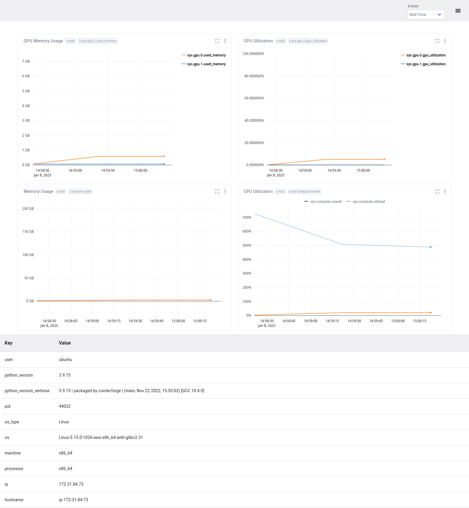
The System Metrics tab display information about your training environment. The page displays four graphs aimed at helping users identify bottlenecks in their training scripts:
- Memory, Power Usage, Temperature and % utilization used by each GPU device.
- Memory usage and CPU utilization.
sys.compute.overallrefers to the percentage of utilization of all CPU cores, whilesys.compute.utilizedrefers to the percentage of utilization for the current training process. Values above 100% are possible through parallelization. - Network utilization, both incoming and outgoing network traffic. Metrics are reported in bytes per second.
- Disk utilization, both total usage and I/O rates.
As models are often trained on large machines, we limit the system metrics logged to the ones used as part of the training process. This is done by checking for the CUDA_VISIBLE_DEVICES environment variable, if it isn't set then all the metrics are logged for each GPU.
Info
Before the Python SDK version 3.31.21, the CPU metrics were the percentage of utilization of each core instead. Those values are still logged and you can visualize them with the built-in Line panel, look for metrics that contain the string sys.cpu.
Below the graphs, there is a section with key-value information about the training environment. This includes details such as the Python version, OS name and version, and other relevant details. This information can help users understand the context in which the training is taking place and troubleshoot any issues that may arise. Here is a list of what is logged automatically by the Python SDK:
| Name | Description |
|---|---|
| user | The OS username |
| python_version | The Python Version as MAJOR.MINOR.PATCh |
| python_version_verbose | The detailed Python Version |
| pid | The process identifier of the process that created the Experiment |
| os_type | The OS type |
| os | The platform name |
| osRelease | The OS release |
| machine | The Machine type |
| processor | The Processor name |
| ip | The IP address of the interface used to connect to Comet |
| hostname | The hostname of the machine |
You can log more data manually by calling Experiment.log_log_system_info or APIExperiment.log_additional_system_info.
Graphics tab
The Graphics tab becomes visible when an Experiment has associated images. These are uploaded using the Experiment.log_image() method in the Python SDK.
Audio tab
The Audio tab shows the audio waveform uploaded with the Experiment.log_audio() method in the Python SDK.
For each waveform, you can hear it by hovering over the visualization and pressing the play indicator. Click in the waveform to start playing at any point during the recording.
Text tab
The Text tab shows strings logged with the Experiment.log_text() method in the Python SDK.
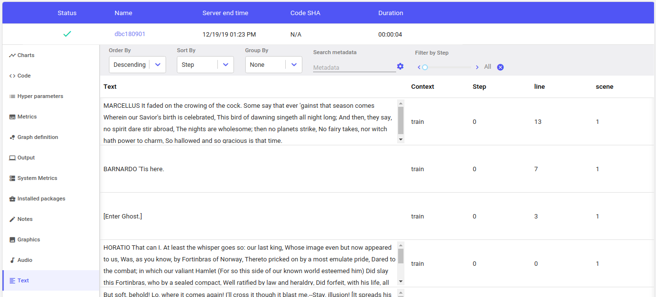
You can use Experiment.log_text(TEXT, metadata={...}) to keep track of any kind of textual data.
Confusion Matrices tab
The Confusion Matrices tab shows so-called "confusion matrices" logged with the Experiment.log_confusion_matrix() method in the Python SDK. The confusion matrix is useful for showing the results of categorization problems, like the MNIST digit classification task. It is called a "confusion matrix" because the visualization makes it clear which categories have been confused with the others. In addition, the Comet Confusion Matrix can also easily show example instances for each cell in the matrix.
Here is a confusion matrix after one epoch of training a neural network on the MNIST digit classification task:
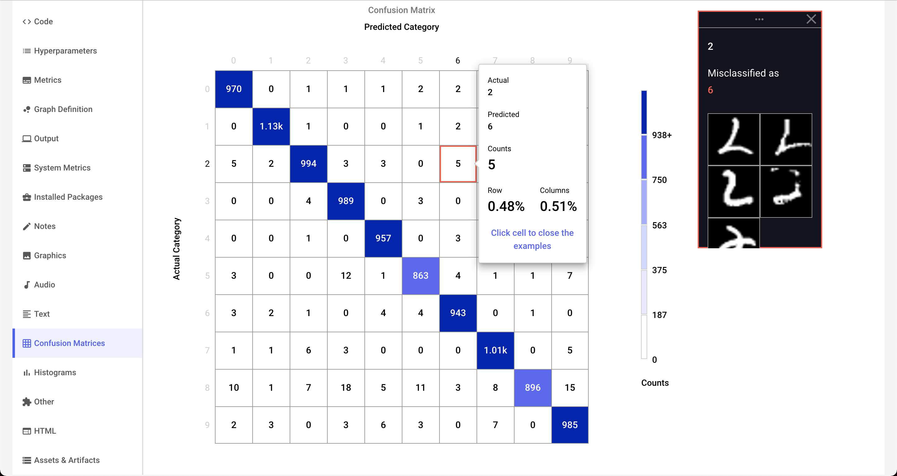
As shown, the default view shows the "confusion" counts between the actual categories (correct or "true", by row) versus the predicted categories (output produced by the network, by column). If there is no confusion, then all the tested patterns would fall into the diagonal cells running from top left to bottom right. In the above image, you can see that actual patterns of 0's (across the top row) have 966 correct classifications (upper, left-hand corner). However, you can see that there were 5 patterns that were "predicted" (designated by the model) as 6's.
If you hover over the 0-row, 6-column, you see a popup window similar to this:
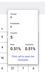
This window indicates that there were five instances of a 0 digit that were confused with being a 6 digit. In addition, you can see the counts, and percentages of the cell by row and by column.
If you would like to see some examples of those zeroes misclassified as sixes (and the confusion matrix was logged appropriately), simply click the cell. A window with examples is displayed:
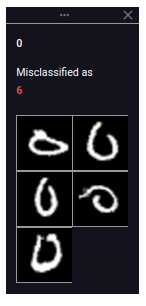
You can open multiple example windows by clicking additional cells. To see a larger version of an image, click the image in the example view. There you will also be able to see the index number (the position in the training or test set) of that pattern.
Some additional notes on the Confusion Matrices tab.
You can:
- Close all open example views by clicking Close all example views in the upper, right-hand corner.
- Move between multiple logged confusion matrices by selecting the name in the upper left corner.
- Display counts (blue), percents by row (green), or percents by column (dark yellow) by changing Cell value.
- Control what categories are displayed (for example, select a subset) using
Experiment.log_confusion_matrix(selected=[...]). - Compute confusion matrices between hundreds or thousands of categories (only the 25 most confused categories will be shown).
- Display text, URLs, or images for examples in any cell.
Histograms tab
The Histograms tab shows time series histograms uploaded with the Experiment.log_histogram_3d() method in the Python SDK. Time series are grouped together according to the name given, and assumes that a step value has been set. Step values should be unique, and increasing. If no step has been set, the histogram will not be logged.
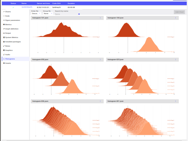
Each histogram shows all of the values of a list, tuple, or array (any size or shape). The items are divided into bins, based on their individual values, and the bin keeps a running total. The time series runs from earliest (lowest step) in the back, to early steps in the front.
Time series histograms are very useful for seeing weights or activations change over the course of learning.
To remove a histogram chart from the Histograms tab, click the chart's options under the three vertical dots in its upper right-hand corner, and select Delete chart. To add a histogram chart back to the Histograms tab, click Add Chart in the view. If it is disabled, that means that there are no additional histograms to view.
HTML tab
You can append HTML-based notes in the HTML tab during the run of the Experiment. You can add to this tab by using the Experiment.log_html() and Experiment.log_html_url() methods from the Python SDK.
Assets tab
The Assets tab lists all of the images, models and other assets associated with an experiment. These are uploaded to Comet by using the Experiment.log_image(), Experiment.log_model() and Experiment.log_asset() methods from the Python SDK, respectively.
If the asset has a name that ends in one of the following extensions, it can also be previewed in this view.
| Extension | Meaning |
|---|---|
.csv | Comma-separated values file |
.js | JavaScript program |
.json | JSON file |
.log | Log file |
.md | Markdown file |
.py | Python program |
.rst | Rust program |
.tsv | Tab-separated values file |
.txt | Text file |
.yaml or .yml | YAML file |
Reproduce an Experiment
Let's say you're a new member of a data science team and you would like to rerun an Experiment to verify results.
Or perhaps you made some changes to your code and they don't work as expected. Now you would like to take your project back to an older state where the results were better.
Comet lets you return to an Experiment that has run and rerun it using the same code, command, and parameters that were used then.
- Display a single Experiment.
- Click Reproduce.
A window is displayed:
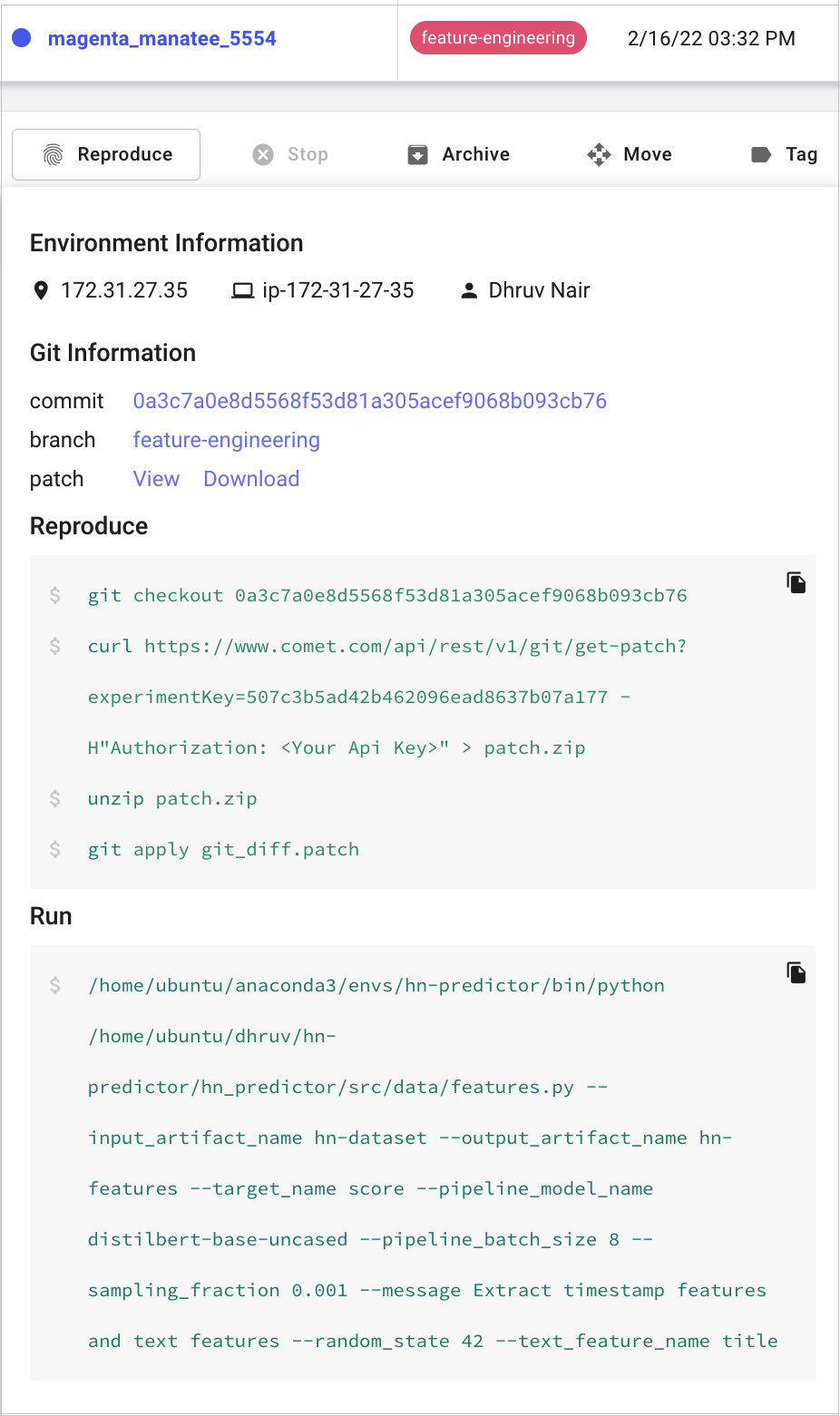
The following information is shown:
- Environment Information: IP, host name, and user name.
- Git Information: Link to the last commit, current branch and a patch with uncommitted changes.
- Run: The command that was used to execute the Experiment.
Info
The set of commands checks out the correct branch and commit. In case there were uncommitted changes in your code when the experiment was originally launched, the patch will allow you to include those as well.
Perform more operations on an Experiment

There are buttons across the top of the Experiment details for performing the following actions:
- Reproduce: See the previous section.
- Stop: Stop an experiment that is running on your computer, cluster, or on a remote system, while it is reporting to Comet. See Stop an Experiment for more details.
- Archive: Soft-delete Experiments. Navigate to the Project Archive tab to either restore or permanently delete your archived Experiments.
- Move: Move your Experiment to another Project. If you choose, the move can be by symbolic link (symlink). In that case, the Experiment remains in the current Project and a reference is added to the target Project.
- Tag: Add a tag to your Experiment. You can also programmatically populate tags with the
Experiment.add_tag()method. To create a new tag, just enter the text and press Enter.